

Unlike stocks or spot FX, trading futures means dealing with something most investors never think about: expiry. Futures don’t last forever. If you want to stay in the trade, you need to roll—close out the expiring contract and open a new one further out on the curve.
That sounds straightforward, but the implications are anything but. Different delivery months come with different liquidity, volatility, seasonal pressures, and supply-demand quirks. Your choice of roll schedule—monthly, quarterly, December-only, front-month—may meaningfully shape your return profile. And in some cases, it defines the behavior of your exposure more than the asset itself.
At Takahē Capital®, we trade over 100 markets and pay close attention to this detail. In our Global Quantitative Fund, we run both outright trend systems and specialized spread strategies, many of which are highly sensitive to month selection. These aren't abstract considerations—they show up in performance, volatility, and curve structure.
Some passive products, like the USO oil ETF, used to roll exclusively in the front month—a method that led to challenges during extreme contango. That practice has since evolved, but the lesson remains: how you roll matters.
This article highlights just a few cases—gas, gasoline, crude oil, wheat—where different roll choices lead to different paths. It’s not about seasonality for its own sake. It’s about knowing where you sit on the curve
🔥 The European Gas Market: A Case Study in Seasonality
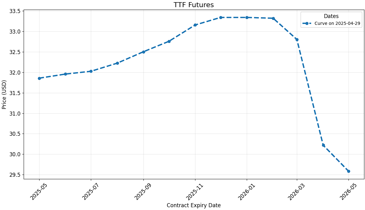
In late 2024, European natural gas markets saw an unusual development: summer 2025 contracts began trading at a premium to winter 2025/26 contracts—a rare instance of seasonal backwardation.
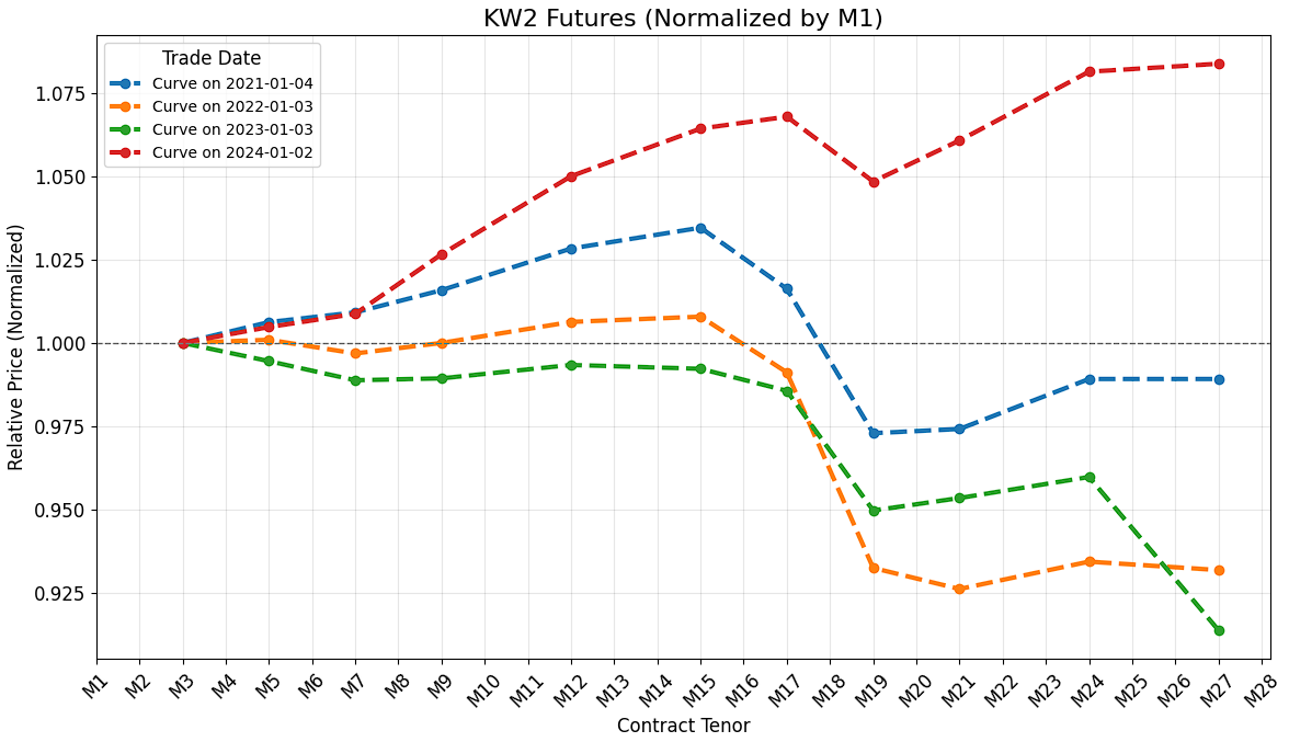
Figure 1 shows the normalized shape of the TTF gas futures curve at year-end (December) across three different years.

The x-axis shows contract tenors, labeled as M1, M2, M3, and so on—these refer to the sequential futures contracts from the trade date:
M1 is the front-month contract (next to expire),
M2 is the following month,
M3 is two months out,
and so on.
This format helps visualize the shape of the curve independent of calendar dates—focusing purely on the structure of future pricing at a given point in time.
2022 and 2023 (blue & orange): clear premium for winter delivery in contrast to the near dated summer months—typical of gas markets recovering from the shock of 2021–2022.
2024 (green): By December 31, 2024, the summer 2025 contract traded ~€4/MWh higher than the winter 2025/26 contract.
This reversal of the usual seasonal structure was driven by:
Several factors contributed to this inversion:
Mandated Storage Refill Targets: The European Union's requirement for member states to fill gas storage to 90% capacity by November 1 led to increased demand for summer contracts, as traders anticipated higher summer gas prices due to the need to refill depleted storage levels.
Speculative Trading: Investment funds and traders speculated on the expected tightness in the summer gas market, taking long positions in summer contracts to capitalize on anticipated price increases. This speculative activity further drove up summer prices relative to winter contracts.
Market Anomalies: The combination of storage mandates and speculative trading led to market anomalies, where summer gas prices exceeded winter prices, disincentivizing storage injections and potentially leading to supply challenges in the subsequent winter.
By early 2025, discussions emerged about relaxing storage mandates to alleviate market distortions. The European Commission considered providing member states with greater flexibility in meeting storage targets to reduce system stress and avoid market disruptions.
As a result of these discussions and changing market dynamics, the summer-winter spread began to normalize, with summer contracts no longer trading at a premium over winter contracts, see figure 2 below. This correction was also influenced by improved weather conditions, increased renewable energy output, and easing geopolitical tensions.
You can't ignore the curve.
⛽ Gasoline: Why Blends and Behavior Matter
Figure 3 below shows the shape of the RBOB gasoline futures curve each January from 2021 to 2024. Prices are normalized to the front-month (M1), so all lines start at 1.0—making it easier to compare relative movements across the curve.

A few patterns stand out:
Spring/Summer Spike (around M3–M7): This reflects the seasonal shift to more expensive summer blends and rising demand as the U.S. driving season approaches. Summer gasoline has tighter environmental specifications and higher production costs, which push futures prices higher in those delivery months.
Autumn Drop-Off (around M9–M13): Demand softens post-summer, and refineries switch back to cheaper winter blends. This is clearly visible as a downward slope or dip in the curve.
Secondary Lift (around M16–M18 and M27–M28): The same seasonal pattern repeats in the second and third years of the curve. Though less pronounced due to long-dated uncertainty, the cycles remain visible.
These futures curves capture how seasonality, regulation, and consumption habits shape the market’s expectations. And they show why rolling summer contracts can look and behave very differently than winter ones—even when the broader trend remains the same.
🌞 Summer vs. ❄️ Winter Rolls: A Tale of Two Tracks
Rolling summer gasoline contracts vs. winter contracts shows how roll schedules influence performance—even when you're trading the same underlying trend.
Figure 4 shows:
Blue: Rolling winter months only
Orange: Rolling summer months only

Path: Summer contracts may experience sharper price moves due to driving season dynamics, refinery switchovers, or regulatory blend changes. Winter contracts might follow a steadier course tied to heating demand or reduced travel.
Volatility: Summer blends often show more price variance due to tighter supply and volatile demand. Winter contracts may be more stable but less reactive.
Carry: The curve can shift—summer contracts may be in backwardation (positive roll yield), while winter months sit in contango (negative roll yield).
Same commodity, but depending on the contract and roll schedule, you're surfing a very different wave.
🛢️ Crude Oil: Smooth on the Surface
Crude oil doesn’t show sharp seasonal curves like gasoline. But that doesn’t mean roll strategy is trivial.
If you look closely at January WTI futures (ticker CL2) curves across multiple years—as shown in figure 5 below—you’ll often see a slight upward kink in the front end of the curve. That lift is typically attributed to post-year-end inventory restocking, early positioning for spring demand, or seasonal hedging activity. But there's more going on under the surface.

That kink is much more pronounced in WTI than in Brent—and the reason lies in delivery logistics.
WTI is delivered inland at Cushing, Oklahoma, a hub with extensive storage infrastructure but limited outbound flexibility. When tanks are full (think "tank tops"), near-term storage becomes expensive, and short-term futures incorporate that cost—known as surge pricing. The futures curve reflects those elevated short-term storage and insurance costs.
Brent, on the other hand, is loaded offshore in the North Sea, where storage is limited. While Rotterdam has capacity, it’s not the official delivery point. This lack of storage pressure means Brent curves typically don’t exhibit the same near-term contango behavior.
There's also a grade dynamic: WTI is a light, sweet crude that's well suited for refining into gasoline (like RBOB), whereas Brent is heavier and sourer, making it more aligned with diesel or gasoil production. These downstream relationships influence how each contract behaves in different seasonal or macro environments.
So while the crude curve may look smooth, those small structural quirks—logistics, storage cost, grade, and delivery point—can have meaningful effects on how different contracts roll, and how strategies perform.
Take a look at figure 6 below. It compares two different rolling strategies applied to the same crude oil trend:
Blue: Rolling monthly
Orange: Rolling once annually in December

Despite tracking the same market, the two paths diverge—sometimes meaningfully.
Monthly rolling introduces more short-term noise, especially around seasonal transitions or inventory data.
December-only rolling smooths out many of those fluctuations. Why? It avoids the spring/fall “shoulder seasons” and benefits from deeper liquidity and hedging flows typically seen in December.
The result:
Monthly rolling: ~34% annualized volatility
December-only: ~28% annualized volatility
Fewer rolls = fewer frictions. However, the choice of roll window can shape your exposure.
🌾 Kansas Wheat: Seasonality You Can See?
Kansas wheat (Hard Red Winter Wheat) has a well-defined production cycle: it’s planted in the fall, lies dormant through the winter, grows in the spring, and is harvested from May to July. You’d expect that seasonality to translate into consistent patterns in the futures curve. But in reality, it doesn’t always work that cleanly.
Figure 7 below shows Kansas Wheat futures curves each January from 2021 to 2024, normalized to the front-month contract. While the crop calendar remains constant, market behavior does not:
In 2021 (blue), the curve steepened notably between March and December —possibly as the market priced in tightening conditions or supply constraints.
In contrast, 2022 and 2023 (orange and green) stayed relatively flat. Droughts eventually did hit both years, but in January those risks probably weren’t yet visible.
A particularly steep curve appears in 2024 (red line)—with far-dated contracts trading significantly above the front. This shape likely reflects rising uncertainty and risk premiums heading into the 2024/25 crop year. By January, early concerns around weather in Russia and worsening crop conditions in Kansas were already starting to influence sentiment. By early spring, reports of drought stress in the U.S. Southern Plains and severe frosts in Russia pushed futures sharply higher. The elevated deferred prices suggested the market was already anticipating a potential supply shock.
Even with a strict crop cycle, the forward curve often prices weather, geopolitics, and emotion—not just biology.
📉 Beyond Roll Schedules: Adjustments, Charts, and Tradeoffs
Once you’ve chosen a roll schedule, you face another reality—how to construct the historical time series. Unlike spot assets, futures contracts change over time. To build a continuous price chart, you need to stitch together contracts. That’s where adjustment methodologies come in.
The two most common are:
Difference adjustment: Subtract the gap between contracts at each roll point. This keeps absolute price levels but often results in negative prices when markets are in long-term contango.
Ratio adjustment: Multiply the previous series by the ratio of old to new price. This preserves relative returns but distorts nominal price levels.
The chart below shows historical prices for the same futures contract (crude oil), adjusted three different ways:
Blue: Ratio-adjusted
Green: Difference-adjusted
Red: Unadjusted (front-month contract)

While all three track the same underlying asset, the visual—and analytical—implications diverge sharply.
The ratio-adjusted series (blue) maintains consistent percentage returns across rolls. But in periods of persistent contango (when each new contract is priced higher than the last), this method multiplies past prices upward with each roll. Over time, this causes historical prices to appear inflated, especially during the 2000s.
The difference-adjusted series (green) applies a (dynamic) subtraction to offset roll gaps. This avoids artificial inflation of past prices, but during strong contango, repeated subtractions can push historical prices sharply downward—and occasionally even negative.
The unadjusted front-month series (red) shows the real market prices as traded, but includes visible jumps at each roll, making it harder to model returns or trends reliably.
Same underlying data—three different realities, depending on how you stitch the rolls.
This is why understanding adjustment methodology isn’t optional. The way you prepare your futures data can fundamentally change what your models "see"—and how they react. It also determines which model you’re actually able to use on the data.
🔚 Wrapping the Curve
Futures trading isn’t just about direction—it’s about structure, mechanics, and nuance. The shape of the curve, the choice of contract, and how you handle rolls and adjustments all shape the truth your model sees. Ignore that, and even the best strategy can drift off course.
At Takahē Capital®, we treat these details as first-order. From trend systems to spread structures, our strategies are built not just to follow markets, but to understand the machinery underneath.
Because in futures, edge doesn’t just come from spotting trends—it comes from knowing how to ride them.
🔍 Learn more at www.takahe.capital